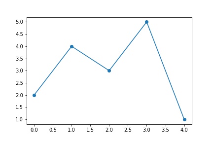
Figure et axes¶

Un graphique consiste en objets

Figure l’espace total du graphique
Axes la partie qui présente les données

Figure¶

La fonction subplots() retourne un tuple consistant de

Figure le conteneur global
Axes pour présenter les données

fig, ax = plt.subplots()

La classe Figure a environ 150 méthodes.

f = [x for x in dir(fig) if not x.startswith('_')]
print(len(f))
f[:20]

['add_artist',
 'add_axes',
 'add_axobserver',
 'add_callback',
 'add_gridspec',
 'add_subplot',
 'align_labels',
 'align_xlabels',
 'align_ylabels',
 'artists',
 'autofmt_xdate',
 'axes',
 'bbox',
 'bbox_inches',
 'callbacks',
 'canvas',
 'clear',
 'clf',
 'clipbox',
 'colorbar']

Taille¶

La taille de la figure par défaut est 6 x 4 pouces.

fig.get_figwidth(), fig.get_figheight()

(6.0, 4.0)

Nous pouvons modifier la taille avec le mot-clé figsize.

plt.subplots(figsize=(8, 2));

Couleur¶

La couleur du graphique est choisie avec facecolor.

plt.subplots(facecolor='lightgray', figsize=(8, 2));

La couleur du contour et son épaisseur peuvent être choisies.

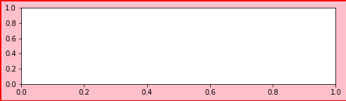
plt.subplots(figsize=(8, 2), facecolor='pink', 
             edgecolor='red', linewidth=3, frameon=True);

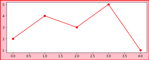
y = [2, 4, 3, 5, 1]
plt.subplots(figsize=(8, 3), facecolor='pink', 
             edgecolor='red', linewidth=3, frameon=True)
plt.plot(y, 'or-');

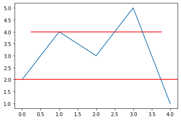
Ligne¶

Des lignes horizontales et verticales peuvent être ajoutées.

plt.plot(y);
plt.axhline(2, c='r')
plt.axhline(4, 0.1, 0.9, c='r');

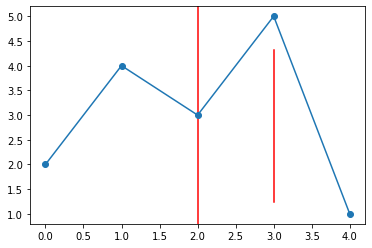
plt.axvline(2, c='r')
plt.axvline(3, 0.1, 0.8, c='r')
plt.plot(y, 'o-');

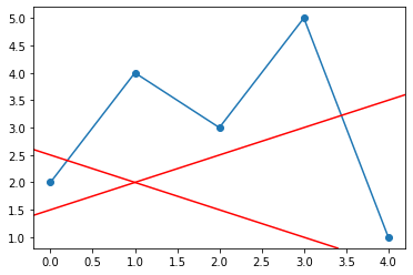
Une ligne d’orientation générale est indiquée avec axline et deux points de référence.

plt.plot(y, 'o-');
plt.axline((1, 2), (2, 1.5), c='r')
plt.axline((1, 2), (2, 2.5), c='r');

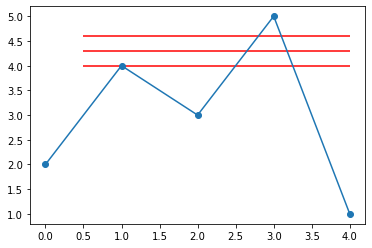
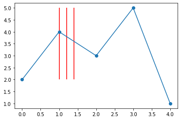
Lignes multiples¶

plt.plot(y, 'o-')
plt.hlines((4, 4.3, 4.6), 0.5, 4, color='r');

plt.plot(y, 'o-')
plt.vlines((1, 1.2, 1.4), 2, 5, color='r');

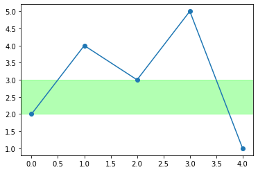
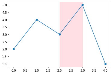
Bandes¶

La méthode axhspan et axvspan permet de placer des bandes horizontales ou verticales.

plt.axhspan(2, 3, alpha=0.3, color='lime')
plt.plot(y, 'o-');

plt.axvspan(2, 3, alpha=0.5, color='pink')
plt.plot(y, 'o-');

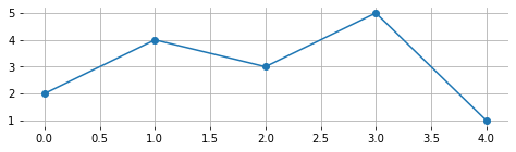
Boîte de contour¶

La boite de contour est optionnelle.

plt.subplots(figsize=(8, 2))
plt.plot(y, 'o-');
plt.box(False)
plt.grid(True)

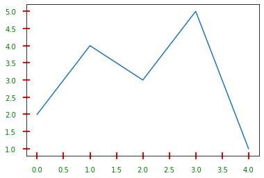
Marques de graduation¶

plt.plot(y, 'o-')
plt.minorticks_on()

plt.plot(y);
plt.box(True)
plt.tick_params(length=10, width=2, direction='inout', 
                color='red', pad=10, labelcolor='g')

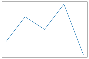
plt.plot(y);
plt.tick_params(length=0, labelleft=False, labelbottom=False)

Valeurs par défaut¶

Toutes les valeurs par défaut sont définis dans rc (runtime configuration).

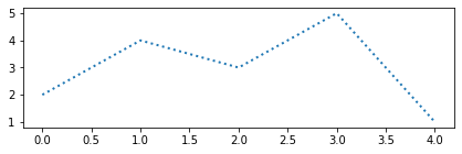
plt.rc('figure', figsize=(7, 2))
plt.rc('lines', linewidth=2, color='r', linestyle=':')

plt.plot(y);

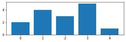
plt.bar(range(5), y);

Axes¶

Les axes ont plus que 300 attributs et methodes.

a = [x for x in dir(ax) if not x.startswith('_')]
print(len(a))
a[:20]

['acorr',
 'add_artist',
 'add_callback',
 'add_child_axes',
 'add_collection',
 'add_container',
 'add_image',
 'add_line',
 'add_patch',
 'add_table',
 'angle_spectrum',
 'annotate',
 'apply_aspect',
 'arrow',
 'artists',
 'autoscale',
 'autoscale_view',
 'axes',
 'axhline',
 'axhspan']

Sous-graphes¶

La fonction subplot(n, m) crée \(n \times m\) sous-graphes.

plt.subplots();

plt.subplots(2, 1);

plt.subplots(1, 2);

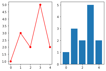
Spécifier un sous-graphe¶

La fonction subplot(n, m, i) sélectionne le i-ième sous-graphique d’une matrice de \(n \times m\) sous-graphes.

Si le nombre des graphes est inférieur à 10 on peut les désigner directement avec subplot(nmi)

x = [0, 1, 2, 3, 4]
y = [1, 3, 2, 5, 2]

plt.subplot(121)
plt.plot(y, 'ro-')
plt.subplot(122)
plt.bar(x, y);

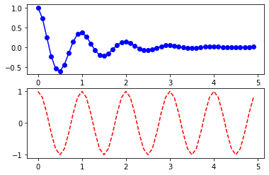
Ici les graphes sont superposés.

t = np.arange(0.0, 5.0, 0.1)

plt.subplot(211)
plt.plot(t, np.exp(-t) * np.cos(2*np.pi*t), 'bo-')

plt.subplot(212)
plt.plot(t, np.cos(2*np.pi*t), 'r--');

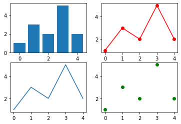
Sous-graphes en 2x2¶

Nous pouvons aussi sous-diviser en \(2 \times 2\) sous-graphes.

plt.subplot(221)
plt.bar(x, y)
plt.subplot(222)
plt.plot(y, 'ro-');
plt.subplot(223)
plt.plot(x, y)
plt.subplot(224)
plt.plot(x, y, 'og');

Arrangement particulier¶

Il est possible de varier le nombre de sous-graphes dans chaque ligne.

plt.subplot(2,1,1)
plt.xticks([]), plt.yticks([])

plt.subplot(2,3,4)
plt.xticks([]), plt.yticks([])

plt.subplot(2,3,5)
plt.xticks([]), plt.yticks([])

plt.subplot(2,3,6)
plt.xticks([]), plt.yticks([]);

Enregistrer une figure¶

La fonction savefig() permet de sauvegarder une figure. L’extension du fichier détermine le format.

y = [2, 4, 3, 5, 1]
plt.plot(y, 'o-');
plt.savefig('img/demo.png')
plt.savefig('img/demo.jpg')
plt.savefig('img/demo.pdf')

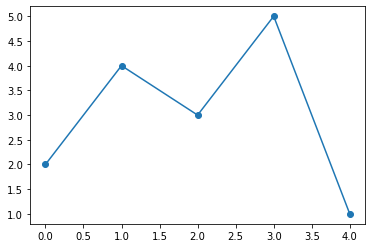
Les trois fichiers se trouvent dans le dossier local. Le PDF est le plus petit, le JPG le plus grand.

ll img/demo*

-rw-r--r--  1 raphael  staff  17497 Jan 17 20:38 img/demo.jpg
-rw-r--r--  1 raphael  staff   5973 Jan 17 20:38 img/demo.pdf
-rw-r--r--  1 raphael  staff  13472 Jan 17 20:38 img/demo.png

L’image peut être affiché dans un notebook avec la commande ![](img/demo.jpg)

Education numérique